This article was first published on Computer Vision News of December 2021
by Ioannis Valasakis @wizofe
Introduction to Neuroscience Image Processing using Jupyter Notebooks
Are you excited about neuroscience and coding with brains? This month it’s all about this. Let’s dive in. Without further ado, I am presenting you NIFTI, NIBABEL but also a short introduction (to be continued in the next issue) of General Linear Models (GLMs).
We’ll start with the required setup, introduction and presentation of data and how to use a Python Jupyter notebook to access and process them.
There’s also an amazing package introduced here, it’s called BData from Kamitani lab (where amazing info was taken from) and here used as a machine learning data format which you can utilize in your later models. Enjoy and feel free to let me know if you use it in your project and how!
Setup
!pip install numpy matplotlib
!pip install nibabel
!mkdir data
!curl https://s3-eu-west-1.amazonaws.com/pfigshare-u-files/27995283/sub01_sesan-atomy_T1w.nii.gz -o data/sub-01_ses-anatomy_T1w.nii.gz
!curl https://s3-eu-west-1.amazonaws.com/pfigshare-u-files/27995286/sub01_sespe-rceptionNaturalImageTest01_taskperception_run01_bold.nii.gz -o data/sub-01_ses-perceptionNaturalImageTest01_task-perception_run-01_bold.nii.gz
!ls data
Introduction
In the neuroscience community, MRI images are often saved, processed, and shared in NIfTI-1 format. The file extension is .nii (uncompressed) or .nii.gz (gzipped). A single NIfTI-1 file can contains either 3-D (spatial) or 4-D (spatial + temporal) MRI image.
More information: https://nifti.nimh.nih.gov/nifti-1/
Visualization of NIfTI images
• Use nibabel to handle NIfTI images: https://nipy.org/nibabel/
• nibabel.load load an NIfTI image as a nibabel image instance.
• To obtain the image as a Numpy array, run np.asanyarray(<img>.dataobje).
import os
import nibabel
import numpy as np
import matplotlib.pyplot as plt
Anatomical MRI image (3-D NIfTI image)
First, we are going to see an anatomical MRI image.
# Load an anatomical MRI image (3-D NIfTI image)
img_t1 = nibabel.load(‘data/sub-01_ses-anatomy_T1w.nii.gz’)
# Extract the image as an array
data_t1 = np.asanyarray(img_t1.dataobj)
data_t1.shape
The loaded image should have shape of (256, 256, 208).
You can check the spatial direction of each dimension of the image array by the following code.
nibabel.aff2axcodes(img_t1.affine)
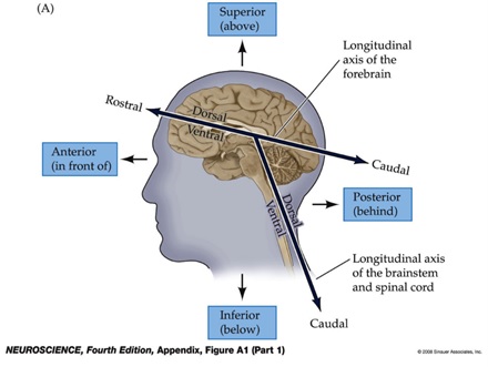
N-th letter represents the incremental direction of N-th dimention of the image array.
• A/P: Anterior/Posterior
• S/I: Superior/Inferior
• L/R: Left/Right
See also: Anatomical terms of location – Wikipedia
Thus, the dimension-direction correspondence of the loaded image is:
• 1st dim: anterior to posterior
• 2nd dim: superior to inferior
• 3rd dim: right to left
Terminology on brain anatomy
• Anterior vs posterior
• Superior vs inferior
• Dorsal vs ventral
You can check the size of each voxel (each element of an MRI image) by the following code (unit: mm).
img_t1.header.get_zooms()
Now, let’s visualize a sagittal slice of the loaded MRI image by display the slice at the center of the left/right axis.
Sagittal, coronal, and axial slices
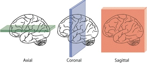
# Visualize the middle sagittal plane
plt.imshow(data_t1[:, :, data_t1.shape[2] // 2].T, cmap=’gray’)
Exercise 1
Visualize axial and coronal planes of the loaded image.
# Axial slice
plt.imshow(<Complete the code>, cmap=’gray’)
# Coronal slice
plt.imshow(<Complete the code>, cmap=’gray’)
Functional MRI image (4-D NIfTI image)
Next, let’s take a look at a 4-D MRI image.
# Load functional MRI images (4-D NIfTI image)
img_fmri = nibabel.load(‘data/sub-01_ses-perceptionNaturalImageTest01_task-perception_run-01_bold.nii.gz’)
# Extract the image as an array
data_fmri = np.asanyarray(img_fmri.dataobj)
data_fmri.shape
You can see that the loaded image is 4-dimensional. The first three dimensions are spatial and the 4th is temporal. So, the image contains whole brain fMRI data from 239 timepoints. The fMRI image at each timepoint is called volume.
Let’s check the dimension-direction correspondence and voxel size.
nibabel.aff2axcodes(img_fmri.affine)
Thus, the dimension-direction correspondense of the loaded image is:
• 1st dim: right to left
• 2nd dim: anterior to posterior
• 3rd dim: inferior to superior
img_fmri.header.get_zooms()
This indicates that the voxel size is mm and each volume was collected at each 2 sec (*).
* Strictly speaking, it takes 2 seconds to collect the data of one volume.
The image size (i.e., the number of voxels) are much less than the anatomical image we investigated above because the spatial resolution of fMRI images is lower than that of anatomical images (i.e., the voxel size of the fMRI image is much larger than the anatomical image).
Let’s visualize a sagittal slice of the first volume in the loaded MRI image.
# Sagittal plane
plt.imshow(data_fmri[data_fmri.shape[0] // 2, :, :, 0].T, cmap=’gray’, origin=’lower’)
Exercise 2
Visualize axial and coronal slices of the first volume in the loaded fMRI image.
# Axial slice
plt.imshow(<Complete the code>, cmap=’gray’)
# Coronal slice
plt.imshow(<Complete the code>, cmap=’gray’)
In 4D fMRI, each voxel is a time series of BOLD signals. Let’s select one voxel and display its time series.
# Time course of a voxel
voxel_index = [33, 78, 42]
plt.imshow(data_fmri[voxel_index[0], :, :, 0].T, cmap=’gray’, origin=’lower’)
plt.plot(voxel_index[1], voxel_index[2], ‘r+’, markersize=12)
resp = data_fmri[voxel_index[0], voxel_index[1], voxel_index[2], :]
plt.plot(resp)
Exercise 3
Calculate temporal mean of the fMRI responses of each voxel, and plot the temporal mean as a brain image (in either sagittal, coronal, or axial plane).
# Complete the code
data_fmri_mean =
plt.imshow()
GLM
This notebook provides brief instruction describing how to run general linear model (GLM) analysis on fMRI data with Python.
Setup
Check if you have not installed the following. If not, you can safely skip them.
!pip install numpy
!pip install nipy
!pip install nilearn
!pip install git+https://github.com/KamitaniLab/bdpy.git
Download data
!mkdir data
# Subject 2
!curl https://ndownloader.figshare.com/files/28089525\?private_link=3bd9a1c29f-19649c8c0d -o data/sub-02_task-localizer_bold_preproc_native.h5
!curl https://ndownloader.figshare.com/files/28089570\?private_link=3bd9a1c29f-19649c8c0d -o data/sub-02_anatomy_t1.nii.gz
!curl https://ndownloader.figshare.com/files/28089528\?private_link=3bd9a1c29f-19649c8c0d -o data/sub-02_template_native.nii.gz
# Subject 3
!curl https://ndownloader.figshare.com/files/28089534\?private_link=3bd9a1c29f-19649c8c0d -o data/sub-03_task-localizer_bold_preproc_native.h5
!curl https://ndownloader.figshare.com/files/28089582\?private_link=3bd9a1c29f-19649c8c0d -o data/sub-03_anatomy_t1.nii.gz
!curl https://ndownloader.figshare.com/files/28089537\?private_link=3bd9a1c29f-19649c8c0d -o data/sub-03_template_native.nii.gz
Import modules
import os
from itertools import product
import bdpy
from bdpy.mri import export_brain_image
import matplotlib.pyplot as plt
import numpy as np
from nipy.modalities.fmri.glm import GeneralLinearModel
from nipy.modalities.fmri.experimental_paradigm import BlockParadigm
from nipy.modalities.fmri.design_matrix import make_dmtx
import nibabel
from nilearn import plotting
fMRI data
In this example, we run GLM analysis on fMRI data collected in the higher visual areas’ localizer experiment. The aim of the experiment is to identify visual areas related to processing of complex visual information such as objects, faces, or scenes. During the experiment, a subject was required to look at an image presented in the scanner. The image was either of them.
• Object images (IntactObject)
• Scrambled version of the object images (ScrambledObject)
• Face images (IntaceFace)
• Scrambled version of the face images (ScrambledFace)
• Scene Images (IntaceScene)
• Scrambled version of the scene images (ScrambledFace)
Example images:
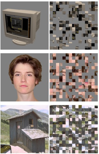
By taking contrast between intact and scrambled images of a particular domain (e.g., IntactObject vs. ScrambledObject), we can get a brain region related to the visual processing of the domain (e.g., lateral occipital complex for object vision).
Here is a list of typical brain regions identified with the experiment.
• LOC (lateral occipital complex; related to object recognition; Malach et al., 1995)
• FFA (fusiform face area; related to face perception; Kanwisher et al., 1997)
• PPA (parahippocampal place area; related to scene perception; Epstein & Kanwisher, 1998)
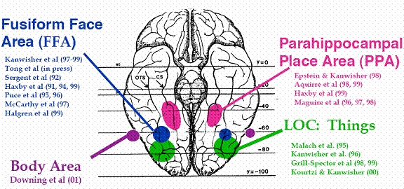
An experiment that identifies a brain region (region-of-interest; ROI) based on the function of the brain (e.g., how voxels are activated by certain stimuli) is called a functional localizer experiment.
Experiment information
• TR: 3 sec
• 100 volumes/run (300 sec/run)
• 8 runs
Blank (24 s) Stim. (15 s) Stim. (15 s) Blank (15 s)
Blank (6 s)
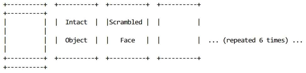
• Stimulus presentation: different images in the category were flashed every 500 ms with blank.
fMRI data format in this example
The fMRI data are saved as BData, machine-learning analysis oriented data format developed in
Kamitani Lab. bdpy is required to read the BData.
bdata = bdpy.BData(‘data/sub-02_task-localizer_bold_preproc_native.h5’)
# Get fMRI data
fmri_data = bdata.select(‘VoxelData’)
fmri_data.shape # volumes x voxels
So the fMRI data are composed of 800 volumes and 32028 voxels.
# Get labels
labels = bdata.get_label(‘block_type’)
np.unique(labels)
The data have nine events. Three of them (‘PreRest’, ‘InterRest’, and ‘PostRest’) are ‘rest’ event in which no visual stimulus was presented. The rest event is not inc luded in the GLM model.
In the other six events (‘IntactFace’, ‘IntactObject’, ‘IntactScene’, ‘ScrambledFace’, and ‘ScrambledObject’), a visual stimulus was presented. These ‘task’ event should be included in the GLM model.
The labels are used to create task regressors, which model the signal changes caused by the experimental conditions (e.g., stimuli).
# Get run numbers
runs = bdata.select(‘Run’)
runs.shape # samplex x 1
This is an array including run numbers, used for creating run regressors, which explicitly model
run-wise fluctuations of the fMRI signals.
Wrapping up!
Amazing work from Kamitani lab where tutorials and the bData package were written! Thanks a lot. All images belong to their respective owners. We claim no rights to any image – please see the sources for more info.
Keep reading the Medical Imaging News section of our magazine.
Read about RSIP Vision’s R&D work on the medical applications of AI.