This article was first published on Computer Vision News of March 2022.
Naronet: Discovery of Tumor Microenvironment Elements from Highly Multiplexed Images
by Ioannis Valasakis
I hope everyone had an amazing time last month and tried out some coding examples from our last issue! As always, feel free to reach out if you have more ideas, examples, requests. Thank you kindly for sending always nice words and suggestions for our future issues.
Let always be kind to people around us, educate and be patient! Keep up the amazing work you are doing in your life, professional and academic world, and most of all: enjoy it.
Review
This month the review article is a very relevant deep learning framework paper, called NaroNet: Discovery of tumor microenvironment elements from highly multiplexed images, published in Medical Image Analysis by Elsevier and authored by Daniel Jiménez-Sánchez, Mikel Ariz, Hang Chang, Xavier Matias-Guiu, Carlos E. de Andrea and Carlos Ortiz-de-Solórzano.
We will try to do our best to review and explain to you in much less detail every article we find interesting from a scientific or exploratory perspective. If you want to learn, go deeper, and understand, even more, remember to always check the original references, article, and have a good discussion about it.
Feel free to share our issue with your friends as well, as this may help evolve to new collaborations, conversations, and disputes (scientific disputes are always the best!)
Introduction
The histopathology and phenotype of a tumor guide its diagnosis, prognosis, and help to predict its response to anticancer treatments. Automating these tasks using machine learning (ML) is the goal of a novel field known as computational pathology. For instance, WSDL has been effectively used for tumor subtyping.
SCA emerged in the context of the research for novel cancer biomarkers. SCA methods build topological networks containing cell phenotype interactions. They apply graph-based clustering to assign groups of cells to different neighborhoods. Since SCA methods use the cell as the basic unit of tissue representation, they provide a high level of interpretability. But you will ask what exactly is this paper trying to do? NaroNet is a multilevel, interpretable deep learning ensemble. It learns the most relevant TMEs from multiplex immunostained tissue sections. It is a computer model that predicts TMEs and predicts clinically relevant parameters and is based on synthetic sets of multiplex images.
Methods and approaches
NaroNet integrates novel and state-of-the-art ML approaches. The development of patch contrastive learning (PCL), a self supervised learning algorithm that encodes high-dimensional pixel information into enriched patch-embeddings. The paper explores the following important elements and is structured as follows: first, the synthetic and real datasets used are explained, followed by the proposed methodology. The next section contains the experiments used to test the performance of NaroNet and reports the results obtained. The following section provides an in-depth analysis of the proposed methods. Finally, the results, conclusions and future ideas are explored.
Let’s see a few of them! First, let’s talk about the data.
Synthetic patient cohorts. An in-house developed multiplex immunostained tissue simulator was used to create patient cohorts. Each patient of the cohort was represented by an 800×800 multiplex image.
7 patient cohorts were simulated. Each cohort contained 240 patients, distributed in 3 groups (type I, II, and III) of 80 patients each with different disease paradigms inspired by real scenarios. Phenotype Marker Intensity (PMI) was used to determine the relative intensity of Mk6 marker expression in each group of patients. Four neighborhoods are defined based on the relative abundance of the phenotypes. Nb3 was set to 15% (moderately present),whereas in PMI2 the relative abundance of Ph6 was set to 0.25% (rarely present).
Phenotype Frequency (PF) was set to 0% (type I), 30% (type II), and 60% (type III) % and in relevant ratios for the other frequencies (you can read in more detail on the paper)
Neighborhood-Neighborhood Interactions (NNI) was designed to simulate different interactions between cellular neighborhoods, related to patient type. Nb2 and Nb3 repel (type I), show no interaction (type II), or attract (type III). Next, tissue sections from twelve high-grade endometrial carcinomas were stained with a seven-color multiplex panel targeting key elements of the immune environment and 336 with a size of 1876x1404x7 pixel images were obtained.
The image dataset is publicly available, and the tissue sections were stained with a 35-plex antibody panel.
Let’s see an image describing the experiment!
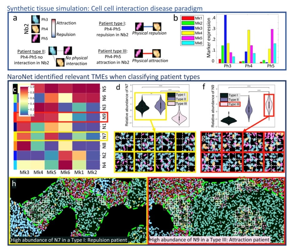
In this figure, you can see the graphical description of the CCI1 experiment. The ground truth on (a) define each patient type which after the processing described earlier leads to classification with the squares showing patches assigned to the learned neighborhood (N9) located in the GT neighborhood Nb2.
The goal of the first step of the pipeline is to convert each high dimensional multiplex image of the cohort into a more manageable list of low-dimensional embedding vectors. To this end, each image is divided into patches – our basic units of representation of the local tissue microenvironment, or phenotype – and each patch is converted by the PCL module.
The PCL module is trained iteratively. In each iteration, the PCL module is unsupervised trained to learn embeddings of a random set of patches. The choice of the image patch size S L is critical as it determines the extent to which biological structures can be captured.
A multi-layer perceptron (MLP) maps each representation to a 128-dimensional vector to create similar embeddings for patches contained in the same crop. A graph is then created that contains all the embedded patches of each tissue/image capturing cellular neighborhoods. This graph is G = (Z, A) where Z is a matrix that contains all the embeddings of the image. A is an adjacency matrix that contains the connectivity between patches.
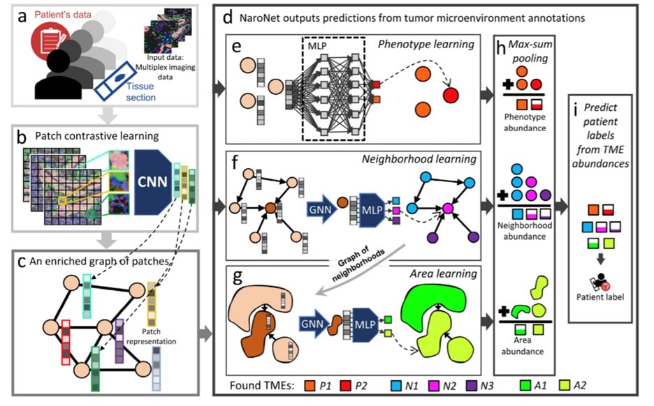
In the previous figure, you can see the process of training NaroNet. It learns a mapping that relates patient information with patient labels. The architecture of NaroNet is divided into two consecutive networks G which is an ensemble of three parallel networks that assigns nodes to distinct P, N, A values. The second section, f2, assigns the patient’s predictions from the learned TMEs. To learn the specific tumor microenvironment, the three neural networks were used with the previously provided data and later pooled to obtain the
abundance of each TME.
Phenotype learning, neighborhood learning (with a graph neural network, GNN) and area learning were utilized as extra elements in the NaroNet.
NaroNet’s classification accuracy (and 95% confidence interval) and interpretability were calculated as the intersection of the most relevant extracted TME and the ground truth of each synthetic experiment. The network parameters and architecture variations are optimally selected by an architecture search algorithm. It identifies elements of the tumor landscape that relate to a specific predictive task. The patient’s predictions are made solely using the relative abundance of TMEs. The model is evaluated with the entire patient cohort, and new prediction probabilities are obtained. If the null hypothesis is accepted, the extracted TME is considered to have a predictive value.
In the following figure, you can see the association of high-grade endometrial carcinomas with patient-level labels. The ROC curves show the classification performance of NaroNet for the four tissue characteristics learned, the neighborhood composition of area A1 and patches assigned to a specific phenotype. Again, see more details of this in the original article!
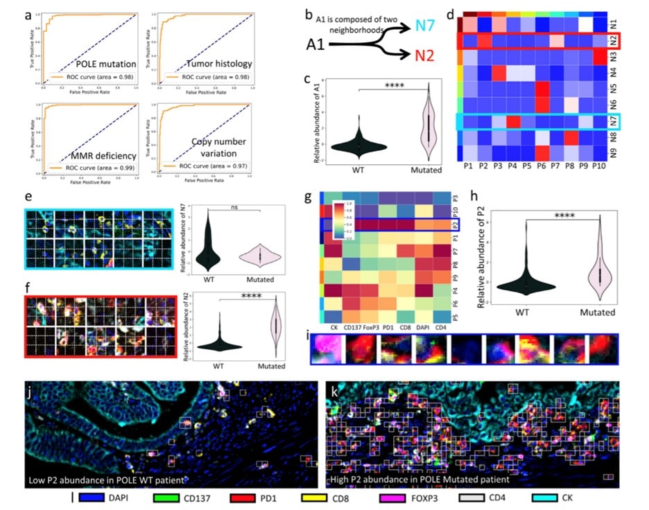
More synthetic experiments were performed on the network, and it was measured on endometrial carcinomas. The network unsupervised learned 26 TMEs. The area A1 (p-value: 2.56×10⁻⁹) seemed the most predictive TME when making patient predictions. A1 is significantly more associated with tumors harboring POLE mutations. To illustrate the individual interpretability of the results, show two examples of images in which phenotype P2 was the most relevant TME selected by NaroNet.
Summarizing
NaroNet is the first WSDL method fully adapted to multiplex imaging. Two state-of-the-art WSDL methods were used to classify H&E tissue sections, adapted for the analysis of multiple images. ClAM is based on a two-step strategy. In the first step, the image is divided into image patches (i.e., hundreds of cells) which are fed to a ResNet50 pre-trained on ImageNet. In the second step, attention scores are assigned to patch representations. NaroNet as an endto-end deep learning framework proves this hypothesis true. It accurately performs patient predictions from local phenotypes, neighborhoods, and areas. One of the major bottlenecks in developing high-performance machine learning classifiers for computational pathology is the low number of available labeled tissue images. A
data-efficient contrastive learning loss pre-processing step was proposed and seem to be efficient.
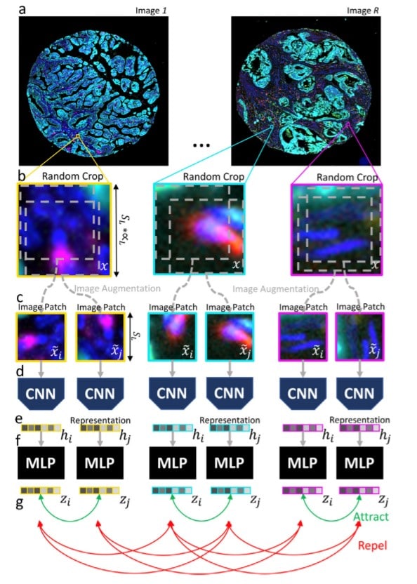
A visualization of the patch contrastive learning is shown on the following image with a step-by-step illustration of the patch contrastive strategy using random crops from the images and CNN which are fed as image patches in a series of CNNs.
NaroNet can learn relevant TMEs local phenotypes, cellinteraction neighborhoods, and neighborhood interaction areas – even when their presence in the tissue is rare.
NaroNet can achieve more accurate predictions while providing inherent interpretability of the reason behind those predictions.
Overall, the network comprises an ensemble of networks that unsupervised identifies and annotates relevant TMEs that drive patient outcomes with clinical predictions which are directly based on the annotations of TMEs.
Keep reading the Medical Imaging News section of our magazine.